
An aquifer is a body of rock or sediment that holds groundwater and transmits enough of it to wells and springs to be useful. The second part of that description is the one that matters for most projects. A great deal of ground holds water. Much less of it will release water at the rate a factory, a data centre or a new township needs, and some of it will deliver water into a basement excavation faster than the design assumed.
This guide covers how aquifers are classified, which properties control their behaviour, how they are investigated and tested, how they respond to excavation and long-term pumping, and what to establish before committing to a site that depends on one. For the wider picture of groundwater and the water cycle, see our guide to how groundwater moves through the subsurface.
What Is an Aquifer?
The US Geological Survey describes a water-bearing rock that readily transmits water to wells and springs as an aquifer (USGS). The definition rests on transmission, not just storage. Confusing the two is a common source of poor decisions.
Aquifers, aquitards and aquicludes
Hydrogeologists group subsurface units by how readily water moves through them. An aquifer transmits water easily enough to supply wells. An aquitard, often clay, silt or shale, transmits water slowly. Over a large area and long periods, an aquitard can still pass significant volumes between the units above and below it. An aquiclude is close to impermeable at the scale being considered.
These categories are relative to the use in question. A silty sand may serve a household borewell well and still behave as an aquitard for an industrial abstraction of several thousand cubic metres a day.
Water in the ground does not mean a productive aquifer
Clay shows the difference. Woessner and Poeter report total porosities for clay of roughly 0.40 to 0.70 but effective porosities of only 0.01 to 0.18 (Woessner and Poeter, 2020). Most of the water is held in pores that do not connect well enough to release it. USGS aquifer maps likewise distinguish minor aquifers that supply little water because they are of local extent, poorly permeable, or both (USGS Principal Aquifers).
A shallow water table therefore says little about water supply. The useful question is whether the formation can deliver water at the required rate, for the required period, without unacceptable effects on neighbours or the environment.
Types of Aquifers: Confinement and Geology
Aquifers are classified along two separate lines: hydraulic confinement, and geology, meaning what the aquifer is made of and where the water is held. The two are often merged in casual descriptions. A sandstone can be unconfined where it outcrops and confined a few kilometres away beneath clay. A granite can behave as unconfined near the surface and as semi-confined at depth beneath a clay-rich weathered layer.
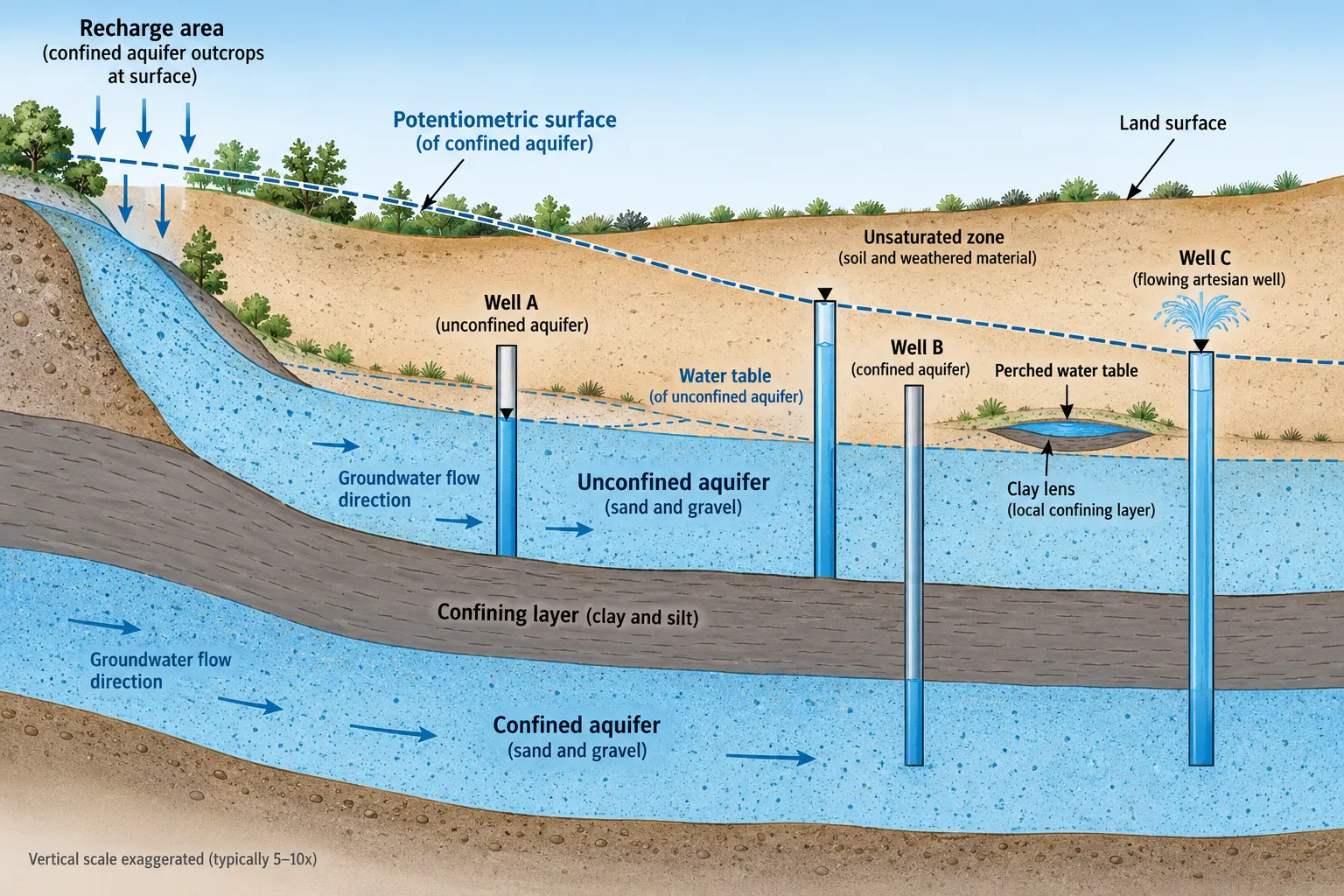
Classification by confinement
Unconfined aquifers have a water table open to the atmosphere through the unsaturated zone above. When a well pumps, pores near the well drain. Each metre of drawdown releases a relatively large volume of water. The US Bureau of Reclamation notes that, for the same rate of extraction, drawdown in an unconfined aquifer is generally smaller and extends over a smaller area than in a confined aquifer (USBR).
Confined aquifers lie beneath a confining layer and hold water under pressure. The water level in a well tapping a confined aquifer rises above the top of the aquifer, and the surface traced by these levels is the potentiometric surface. Pumping lowers the pressure while the aquifer stays saturated. Relatively little water is released per metre of pressure decline, a point developed in the next section.
Leaky or semi-confined aquifers are bounded by layers that still pass some water. Pumping draws water vertically through the aquitard from adjacent units. Leakage can support yield, but it can also draw shallower water of different quality downwards.
Perched groundwater collects on a local low-permeability lens above the main water table. It is often seasonal and limited, rarely a dependable supply, but a common source of unexpected inflow in shallow excavations.
Classification by geology
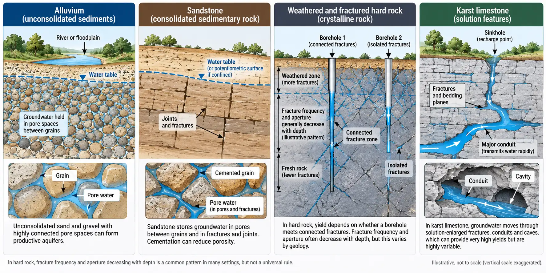
Alluvial and unconsolidated sedimentary aquifers consist of sands and gravels deposited by rivers, deltas and coastal processes, with water held between grains. They can be productive but are usually layered, with clays and silts between the sands. The Gulf Coast aquifer system beneath Houston is a layered system of this kind (HGSD).
Consolidated sedimentary aquifers, such as sandstones and limestones, store water in pores and fractures. Cementation can reduce primary porosity substantially, leaving fractures to control yield in many cases.
Fractured crystalline aquifers, in granite, gneiss and basalt, hold water mainly in fractures. Compiled measurements give fresh granite and gneiss a specific yield below 0.1 per cent, rising to roughly 0.5 to 5 per cent where weathered (Woessner and Poeter, 2020). Storage is limited, and yield depends largely on whether a borehole intersects a connected fracture network. That is why fracture and fault mapping is worth carrying out before drilling locations are fixed.
Weathered hard-rock aquifers are common across much of peninsular India. A weathered zone near the surface stores water, while joints and fractures in the rock below control movement at depth. CGWB aquifer mapping reports often describe a shallow aquifer (Aquifer-I), characterised from weathered zone thickness, and deeper aquifers (Aquifer-II), characterised from exploratory wells (CGWB, Sheopur district report). Airborne electromagnetic surveys in Rajasthan have mapped a weathered and fractured aquifer system compartmentalised beneath alluvial cover (Chandra et al., 2016).
Karst aquifers form where dissolution enlarges fractures in limestone or dolomite into conduits. Flow can be rapid and concentrated, and the laminar-flow assumption behind Darcy's law may not hold in large conduits.
Multilayer aquifer systems
Many large aquifers are stacks of units with different heads, water qualities and properties. A well screened across several units can connect layers that were previously separated. Investigations in these systems need head measurements in each unit, not a single water level.
| Aquifer type | Where water is held | Typical response to pumping | Common engineering concern |
|---|---|---|---|
| Unconfined | Pores below the water table | Pores drain, smaller drawdown footprint | Seasonal yield change, shallow inflow |
| Confined | Pores under pressure | Pressure declines over a wider area | Uplift beneath excavations, interference at distance |
| Leaky | Pores, with flow through aquitards | Drawdown slows as leakage develops | Induced flow from shallower units |
| Perched | Above local low-permeability lenses | Small volume, depletes quickly | Unexpected shallow inflow |
| Fractured crystalline | Fractures | Highly variable between wells | Uncertain yield, preferential contaminant paths |
| Weathered hard rock | Weathered zone and fractures | Yield can fall as the weathered zone drains | Seasonal decline |
| Karst | Dissolution conduits | Localised, sometimes non-Darcian | Rapid contaminant transport, sinkholes |
Aquifer Properties That Control Water Availability
Almost every estimate of well yield, excavation inflow or long-term drawdown depends on hydraulic conductivity, transmissivity and storativity. Each can vary by orders of magnitude, and the values chosen often influence the conclusion more than any other input.
Porosity, effective porosity, specific yield and specific retention
Total porosity (n) is the fraction of a material's volume occupied by voids. Effective porosity (nₑ) counts only the interconnected voids that take part in flow. It can equal total porosity but never exceed it (Woessner and Poeter, 2020).
When a saturated material drains under gravity, only part of the water leaves. The volume drained per unit total volume of material is the specific yield (Sᵧ). Woessner and Poeter define specific retention (Sᵣ) as the water retained in the interconnected pore space after gravity drainage. Under that convention, nₑ = Sᵧ + Sᵣ; because specific retention is non-negative and effective porosity cannot exceed total porosity:
This relationship follows the definitions used by Woessner and Poeter (2020). Other references may define or measure effective porosity and retained water differently, so published values should be read with the source's convention in mind. The practical point does not change. Specific yield, not total porosity, governs how much water an unconfined aquifer gives up as the water table falls. In fine-grained materials the difference is large.
As an illustration, consider 1 km² of unconfined sand with a total porosity of 0.30 and a specific yield of 0.20. A 4 m fall in the water table affects 4,000,000 m³ of ground that held about 1,200,000 m³ of water, but only about 800,000 m³ drains. Supply estimates based on porosity overstate the available water. Hypothetical values.
Hydraulic conductivity and permeability
Hydraulic conductivity (K, m/s or m/day) describes how readily water passes through a material. Intrinsic permeability (k, m²) is a property of the material alone. They are related through the density (ρ, kg/m³) and dynamic viscosity (μ, Pa·s) of the fluid and gravitational acceleration (g, m/s²):
Density and viscosity vary with temperature and salinity, so K for one material varies slightly with the groundwater it carries.
Hydraulic conductivity spans around 13 orders of magnitude across natural materials (Woessner and Poeter, 2020). Knowing K to within an order of magnitude is often useful, and values reported to several significant figures suggest more precision than field methods provide. Two deposits both logged as gravel can differ by orders of magnitude if one is clean and the other contains sand and silt.
Darcy's law and groundwater velocity
Darcy's law relates flow to the hydraulic gradient:
Q is volumetric flow (m³/s), A is the cross-sectional area of flow (m²) and dh/dl is the hydraulic gradient (dimensionless). The negative sign indicates flow towards lower head. The law assumes laminar flow through a saturated porous medium. It may not hold in large open fractures or karst conduits.
Water moves only through the connected pores, so its average speed is higher than the Darcy flux. The average linear (advective) pore-water velocity is:
where v is in m/s and i is the hydraulic gradient. This is a representative average for a volume of aquifer, not the speed of water in any individual pore. Pore-scale velocities vary widely, which spreads dissolved substances out (Woessner and Poeter, 2020).
The equation should not be read as the speed of every contaminant. Dispersion means some of a dissolved substance arrives earlier than the average predicts. Many substances are slowed by sorption to aquifer materials or are degraded along the way. Fractured and dual-porosity media can carry water much faster in fractures than the bulk average suggests. Contaminant travel time estimates need transport analysis, not this equation alone.
Transmissivity and saturated thickness
Transmissivity (T, m²/day) describes the capacity of the full saturated thickness (b, m) to transmit water:
A sand with K of 20 m/day and 15 m saturated thickness has a transmissivity of 300 m²/day (hypothetical values). The relationship assumes K is representative of the full thickness. Layered aquifers can be represented by summing T for each layer.
In a confined aquifer, b stays constant while the aquifer remains saturated. In an unconfined aquifer, b is the distance from the water table to the aquifer base, so transmissivity falls as the water table falls (Woessner and Poeter, 2020). This is one reason wells in shallow unconfined or weathered aquifers often lose yield in the dry season.
Storativity and specific storage
Storativity (S), also called the storage coefficient, is the volume of water released per unit area of aquifer per unit decline in head. It is dimensionless. Confined and unconfined aquifers release water in different ways:
Sₛ is specific storage (per metre), which reflects compression of the aquifer skeleton and expansion of water as pressure falls. In unconfined aquifers gravity drainage dominates, so S is usually taken as Sᵧ (Woessner and Poeter, 2020).
Published ranges differ between texts. Woessner and Poeter give typical confined storativities of 10⁻⁵ to 10⁻³ and typical specific yields of 0.05 to 0.40. Todd gives most confined values as falling between 5 × 10⁻⁵ and 5 × 10⁻³ (Todd, 1980, via NRC exhibit).
How far pressure changes travel
The contrast in storativity explains why confined aquifers can transmit pressure changes over large distances. The ratio of transmissivity to storativity is the hydraulic diffusivity:
D has units of m²/day. A higher diffusivity means a head change moves through the aquifer faster. For one-dimensional flow, the time for a pressure pulse to reach a given distance increases with the square of that distance and decreases as diffusivity increases (Wang, 2020). Because confined storativity is small, a confined aquifer with the same transmissivity as an unconfined one has a much higher diffusivity.
That does not mean pressure effects spread without limit. How far drawdown reaches, and how large it is, depends on how long pumping continues, on leakage through confining layers, and on boundaries such as rivers, faults or the edge of the aquifer, which can limit, redirect or amplify the response. Distance-drawdown predictions for a specific site need site values of T and S and an understanding of its boundaries.
Volume released from storage
The volume released for a head change (Δh, m) over an area (A, m²) is:
Lowering the head by 1 m over 1 km² releases about 100 m³ from a confined aquifer with S = 10⁻⁴, and about 150,000 m³ from an unconfined aquifer with Sᵧ = 0.15. Hypothetical values.
This calculation is a simplification. It assumes a single storativity and a uniform head change across the area. For a confined aquifer, it applies only while the head stays above the top of the aquifer. Below that point the aquifer starts to drain and behaves as unconfined. In an unconfined aquifer, drainage can lag behind the fall in the water table, so the full specific yield may be reached only after some time. The calculation also ignores inflows such as recharge and capture during the period considered. Above all, it describes a change in storage, not a sustainable supply, a distinction covered in the section on well performance.
Heterogeneity, anisotropy and fracture connectivity
Real aquifers are neither uniform nor equally permeable in every direction. Layered sediments commonly transmit water more readily along the bedding than across it. In fractured rock, the property that matters most is often whether fractures connect with each other and with a source of recharge.
Consider two industrial plots three kilometres apart in hard-rock terrain. One borewell meets a fracture zone connected to a weathered layer that is recharged each monsoon, and yields steadily. The other meets isolated fractures, performs well during a short test, then declines as those fractures drain. On a regional map both plots sit on the same granite gneiss unit. Illustrative scenario, not a documented case.
Aquifer properties are not well performance
A poorly performing well does not prove a poor aquifer. Yield also depends on screen design, well development, partial penetration and energy losses as water enters the well, which the step-drawdown test described below helps separate.
Values quoted in this section are representative ranges for illustration, not predictions for any site. Field testing is the reliable source of site values.
Investigating an Aquifer: Mapping and Characterisation
None of these properties can be read from a geological map. They are inferred from evidence gathered in stages, and an investigation works best when designed around the decision it must support, whether a supply of 500 m³/day, a three-level basement or a land acquisition.
Desk study and existing data
Investigations start with existing maps, borehole logs, water-level records, nearby abstraction and regulatory classification. USGS lists these among the data needed to analyse a groundwater system and notes that some, such as long water-level records, exist only if someone collected them years earlier (USGS Circular 1186).
In India, the Central Ground Water Board took up national aquifer mapping under the XII Five-Year Plan, with hydrogeological investigation at 1:50,000 scale (CGWB). District reports, such as the 2023 Mayurbhanj report (CGWB), are a sensible starting point for an Indian site. They are regional, though, and a single industrial plot can sit on conditions the regional map does not resolve.
Geophysics and its limits
Electrical resistivity and electromagnetic surveys map contrasts in the physical properties of the ground. They help trace clay layers, weathered zone thickness, buried channels and fresh-saline boundaries, and can provide indirect indicators of salinity, groundwater quality and geological conditions. They cannot independently establish water quality, hydraulic conductivity or sustainable well yield. A low resistivity can indicate clay, saline water or both. Interpretations need calibration against boreholes. In the Paris Basin, for example, an airborne electromagnetic survey was calibrated against about 50 boreholes before aquifer layers were interpreted in three dimensions (Martelet et al.).
Drilling, logging and observation wells
Drilling provides direct evidence of lithology, water strikes and water levels. Piezometers at several depths show whether different units have different heads, which is critical in multilayer and confined systems. Observation wells at known distances from a pumped well are needed to estimate storativity. A test measured only in the pumping well cannot separate aquifer behaviour from well losses.
Building the conceptual site model
Characterisation produces a conceptual site model: a description of geometry, boundaries, properties, recharge and discharge, and how they interact. A defensible model also states its uncertainty. A model based on two boreholes across a 50-hectare site should say how much of the ground between them is inferred.
| Method | What it can establish | What it cannot establish alone |
|---|---|---|
| Desk study and regional mapping | Regional geology, aquifer units, water-level trends | Site-specific yield or properties |
| Resistivity and electromagnetic surveys | Layer geometry, clay and weathered zone thickness, saline interfaces and other indirect indicators of geological conditions or groundwater quality | Water quality, hydraulic conductivity or sustainable well yield independently |
| Exploratory drilling and logging | Lithology, water strikes, layer depths | Continuity between boreholes |
| Multi-level piezometers | Head in each unit, vertical gradients | Hydraulic properties |
| Pumping tests with observation wells | T, S, leakage, boundary effects | Behaviour beyond the test's area of influence |
| Water sampling | Quality at the time of sampling | Future quality under pumping |
Aquifer Productivity, Pumping Tests and Well Performance
Pumping shows how an aquifer actually behaves. A well-designed pumping test is the most direct way to estimate transmissivity, storativity and the influence of boundaries, and a US EPA guidance note describes it as the most reliable type of aquifer test usually conducted (Osborne, US EPA, 1993). Its results are also easy to misread.
What a pumping test measures
A step-drawdown test pumps a well at a series of increasing rates. How drawdown grows with rate helps separate losses in the well from losses in the aquifer and helps select an operating rate. A constant-rate test pumps at a steady rate while water levels are measured in the pumping well and observation wells, and is the main basis for estimating T and S. A recovery test tracks water levels after pumping stops.
There is no universal duration. Waikato Regional Council in New Zealand treats 24 hours as a general minimum for a constant-rate test, states that tests should continue long enough to show the effects of the proposed pumping, and asks for recovery monitoring for a period similar to the test or until levels return to their starting point (Waikato Regional Council). Local regulators may set their own requirements.
Interpreting results, and where standard methods fall short
Most analyses use the Theis solution (Theis, 1935) or the straight-line simplification of Cooper and Jacob (1946). Both assume an idealised confined aquifer: uniform thickness, homogeneous and equally permeable in all directions, infinite in extent, and fully penetrated by the pumped well. The Cooper-Jacob simplification applies only after pumping has continued long enough for a given distance from the well. USGS emphasised in 1962 that these assumptions limit where each method is valid (Ferris et al., 1962).
| Setting | How results can depart from a Theis fit | More suitable approach |
|---|---|---|
| Fractured rock | Flow concentrates in connected fractures, and drawdown can follow patterns the Theis model does not describe | Fracture mapping before test design, diagnostic plots, fracture-flow or dual-porosity solutions |
| Layered or heterogeneous | Pumping induces vertical flow, so a single K can misrepresent individual layers | Multi-level observation wells, calibrated numerical models |
| Leaky | Drawdown slows or stabilises as leakage develops. Fitting Theis or Cooper-Jacob to the later data can bias T and S | Leaky-aquifer solutions, monitoring of the adjacent unit |
| Unconfined | Delayed drainage. Early data reflect elastic storage and can give a storage value far below Sᵧ | Delayed-yield solutions, longer tests |
| Near a boundary | A recharge boundary flattens drawdown. A barrier steepens it | Image-well analysis, geological mapping of boundaries |
ASTM D5270 notes that the effects of a constant-head boundary are often indistinguishable from those of a leaky confined aquifer, and that locating an unknown boundary requires at least three observation wells (ASTM D5270). A study using simulated three-dimensional tests also concluded that Theis-based conductivity values are unsuitable for two-dimensional models where anisotropy and layering are present (Freed, 2012).
Test analysis produces estimates that fit an assumed model, and a different model can sometimes fit the same data. Geology, test duration and observation wells narrow the choice.
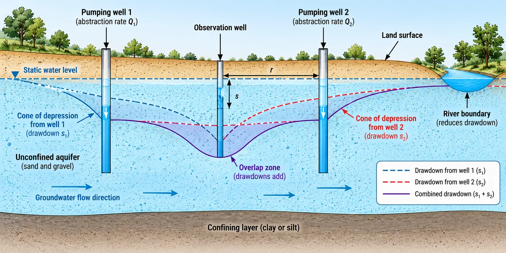
Well interference and boundaries
Under approximately linear aquifer-flow conditions, drawdowns from neighbouring pumping wells can be estimated using the principle of superposition. On a shared aquifer, one abstraction can therefore lower water levels at others. On an industrial estate where several units each drill a borewell, wells that tested well individually can underperform once all are pumping, because no single test captured the combined effect. Illustrative scenario. Boundaries act similarly: a short test may not reach the edge of a narrow alluvial channel or a fault, but sustained pumping can.
Tested yield, aquifer productivity and sustainable abstraction
These terms answer different questions and should not be used interchangeably.
| Term | Question it answers | Main evidence | What it does not tell you |
|---|---|---|---|
| Tested well yield | What rate did this well sustain during this test? | Step-drawdown and constant-rate tests | Long-term behaviour, effects on others, distant boundaries |
| Aquifer productivity | How readily does the formation transmit and release water across the area? | T and S from tests with observation wells, geology | How much can be taken without unacceptable impacts |
| Sustainable abstraction | What total withdrawal can continue without unacceptable environmental, economic or social effects? | Capture analysis, monitoring, models, regulation | A single fixed number |
The concept linking them is capture. USGS explains that when pumping starts, all the water comes from aquifer storage. Over time the source shifts towards capture: water that would otherwise have discharged to streams, springs and wetlands, or water drawn in from them. The transition can take weeks, years or decades (USGS Circular 1186).
For the same reason, natural recharge alone does not set how much can be pumped. USGS calls that idea the water-budget myth, after Bredehoeft and colleagues (1982), and notes that a predevelopment water budget does not show where pumped water will come from (USGS Circular 1186). Sustainable abstraction depends on how the aquifer responds to development and on which effects regulators and society accept, which makes it partly a hydrogeological question and partly a regulatory one.
Aquifers and Excavation: Pressure, Inflow and Uplift
The same properties determine how an aquifer responds when a deep excavation is made in or above it. For basements, metro boxes, pump stations and plant rooms, the aquifer acts as a load on the works rather than a resource.
Piezometric head
For excavation design, the depth to the water table is often less informative than the piezometric head in each permeable unit below formation level. A confined sand 15 m below ground can carry a head close to the surface. An excavation that stops a few metres above that sand may appear dry on a borehole log while sitting above a layer under significant upward pressure. Heads change with season, tide and neighbouring pumping, so a single dry-season reading may not represent construction conditions.
Inflow and seepage
Inflow depends on the transmissivity of the units exposed or underlain, the head difference, the distance to recharge boundaries and the effectiveness of any cut-off. A thin, permeable gravel lens can deliver more water than a thicker fine sand, so geometry matters as much as material properties.
Hydraulic uplift and basal heave
Several failure mechanisms at an excavation base involve groundwater, and they are easily confused.
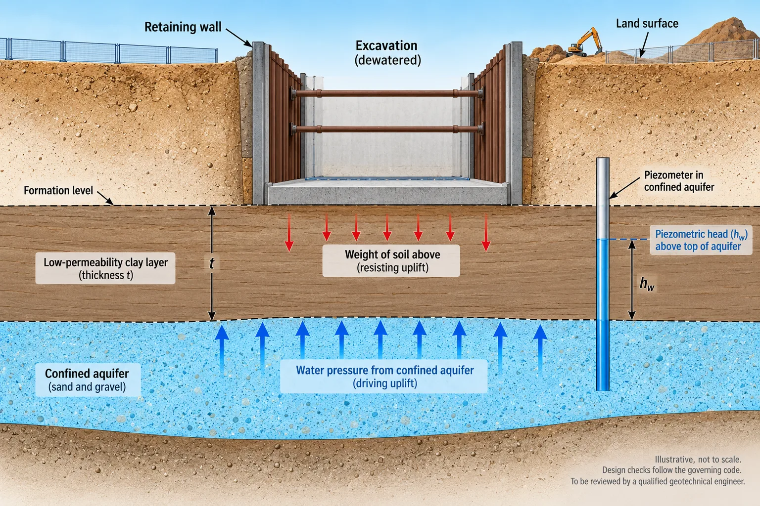
Hydraulic uplift occurs when water pressure in a confined layer beneath the excavation exceeds the resistance of the low-permeability soil above it. The base can lift, crack and flood.
Piping and boiling occur where upward flow through sand beneath an excavation reaches a gradient sufficient to carry particles with it.
Basal heave in soft clay is a shear failure driven largely by the weight of the retained ground. Groundwater affects it, but the mechanism differs from hydraulic uplift.
The mechanism of hydraulic uplift can be illustrated by comparing the weight of the soil above a confined layer with the water pressure at its top:
γ_soil and γ_w are the unit weights of soil and water (kN/m³), t is the thickness of low-permeability soil between formation level and the top of the confined layer (m), and h_w is the piezometric head above the top of that layer (m).
This ratio is included only to show why pressure matters. It is not a design method and should not be used to check an excavation. Design verification must follow the code and specification governing the project, using measured piezometric levels and the factors required by that code. A secondary study of Eurocode 7 HYD provisions reported that two permitted formulations produced different global safety factors for the same excavation (Dołżyk and Szypcio, 2013). The applicable standard text has not been independently checked for this draft, so this is not a completed Eurocode verification. Projects in India, the United States and the UAE require assessment against the codes and specifications governing the project by a qualified geotechnical engineer. Wall friction, the shear strength of the soil plug, excavation width, leakage through walls and changing heads all affect the real margin.
Dewatering, drawdown and settlement
Lowering groundwater reduces pore water pressure around an excavation and increases effective stress, so soft clays, silts and organic soils compress. Buildings, pipes and roads within the zone of influence can settle, sometimes unevenly. Dewatering can also lower water levels in neighbouring wells, and in confined aquifers the depressurised zone can extend beyond the site boundary, subject to the diffusivity, leakage and boundary effects described earlier. Dewatering design for deep excavations therefore starts from the aquifer's geometry and properties and assesses effects on neighbours before pumping begins.
Monitoring during construction
Piezometers below formation level, settlement points on adjacent structures, neighbouring wells and discharge records turn design assumptions into evidence, with trigger levels agreed before excavation starts.
| Risk | Mechanism | Early warning signs | Typical responses |
|---|---|---|---|
| Excess inflow | Permeable layers, nearby recharge boundary | Discharge above prediction, running sand | Additional wells, cut-offs, review of geology |
| Hydraulic uplift | Pressure in a confined layer exceeds resistance of soil above | Rising piezometers below formation, cracking | Depressurisation, relief wells, staged excavation |
| Piping or boiling | High upward gradient in sand | Sand boils, turbid seepage | Reduce gradient, filters |
| Settlement of neighbours | Increased effective stress | Movement at settlement points | Reduced drawdown, recharge wells, cut-offs |
| Interference with wells | Overlapping drawdown | Falling levels in neighbouring wells | Agreed monitoring and mitigation |
Aquifer Vulnerability to Contamination
The connected pathways that let an aquifer transmit water also let it transmit contaminants. Vulnerability describes how readily contamination from the surface could reach an aquifer, based on the ground above and the aquifer itself rather than on a particular pollutant.
Thick, continuous clay over a confined aquifer offers substantial protection, while a shallow water table in coarse sand offers little. Index methods score these conditions. DRASTIC, developed by Aller and colleagues for the US EPA in 1987, rates seven factors: depth to water, recharge, aquifer media, soil media, topography, impact of the vadose zone and hydraulic conductivity (SFU summary of Aller et al., 1987). Such indices compare areas. They are relative measures, have known difficulties with leaky and stacked aquifers, and do not replace site investigation.
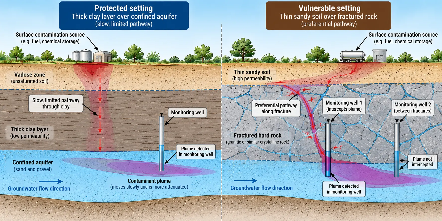
In fractured and karst aquifers, contaminants follow the most connected pathways, and a plume can bypass monitoring wells drilled into less permeable rock between fractures. Designing groundwater monitoring networks around the conceptual site model rather than a regular grid reduces that risk. Where contamination has occurred, aquifer properties also shape the approach to restoring a contaminated aquifer.
Recharge Potential and Storage Limits
Whether an aquifer can usefully accept more water, natural or managed, is a question about the aquifer as well as about rainfall.
Several limits apply. There must be storage space, which in an unconfined aquifer depends on the unsaturated thickness and the specific yield, so a shallow water table leaves little room. Water must be able to infiltrate through soils and the unsaturated zone. Recharge water must be compatible with the aquifer, because reactions and suspended solids can clog infiltration surfaces and wells. And recovered water may differ from the water recharged because the two mix.
Recovery of groundwater levels can reverse some effects of over-abstraction. In Delhi's Dwarka area, satellite radar showed a shift from subsidence to uplift between 2014 and 2020, which the study's authors attributed to stricter regulation of groundwater use and incentives for rainwater harvesting, while noting that detailed hydrogeological analysis was needed to confirm it (Garg et al., 2022). Design of groundwater recharge planning needs site testing of infiltration, storage and water quality.
Aquifer Stress, Compaction and Subsidence
Pumping initially draws water from aquifer storage while capture develops through induced changes in recharge and discharge. Groundwater heads may continue declining during that adjustment. The long-term response depends on pumping rates, aquifer storage, boundaries, recharge and how pumping changes discharge to streams, springs and wetlands. In layered systems with compressible clays, sustained head decline can affect the ground surface.
Falling heads increase the effective stress on clays within and between aquifers. Clays compact slowly, and much of that compaction is not recovered if heads later rise. The land surface subsides, and the aquifer system loses part of its capacity to store water.
Houston is one of the best-documented examples in the United States. USGS reports more than 10 feet of subsidence near Pasadena between 1906 and 1995, with almost 3,200 square miles subsiding by more than 1 foot, mainly because of aquifer-system compaction caused by groundwater pumping. Consequences included more frequent flooding, damage to industrial and transport infrastructure, and fault movement affecting buildings and highways (USGS Fact Sheet 110-02). Where pumping was reduced by switching to surface water, subsidence largely abated. Inland areas still reliant on groundwater continued to subside. The Harris-Galveston Subsidence District, created by the Texas Legislature in 1975, describes subsidence as irreversible once it occurs (HGSD).
India shows the same processes. Satellite gravity data indicated groundwater depletion at a mean rate of 4.0 ± 1.0 cm of water per year over Rajasthan, Punjab and Haryana (including Delhi) between August 2002 and October 2008, equivalent to a net loss of 109 km³ (Rodell et al., 2009). In Delhi NCR, radar analysis for 2014 to 2020 measured subsidence exceeding 11 cm per year in Kapashera, near Indira Gandhi International Airport, and 3 cm per year in Faridabad, with both following the trend of falling groundwater levels (Garg et al., 2022).
For an industrial or infrastructure owner, a declining aquifer creates risk before any well runs dry: deeper pump settings and higher energy use, falling yields as saturated thickness shrinks, changing water quality, tighter abstraction controls and ground movement. Responses often require basin-scale water planning rather than a single-site fix.
Aquifer Models: What They Can and Cannot Predict
Every judgement about an aquifer rests on a model of some kind. A conceptual model describes the system in words and diagrams. Analytical models, such as the Theis solution, give exact answers for idealised conditions. Numerical models divide the aquifer into cells or elements and solve groundwater flow equations across complex geometry, layering and boundaries. MODFLOW 6, the sixth core version of the MODFLOW code, is distributed by USGS (USGS).
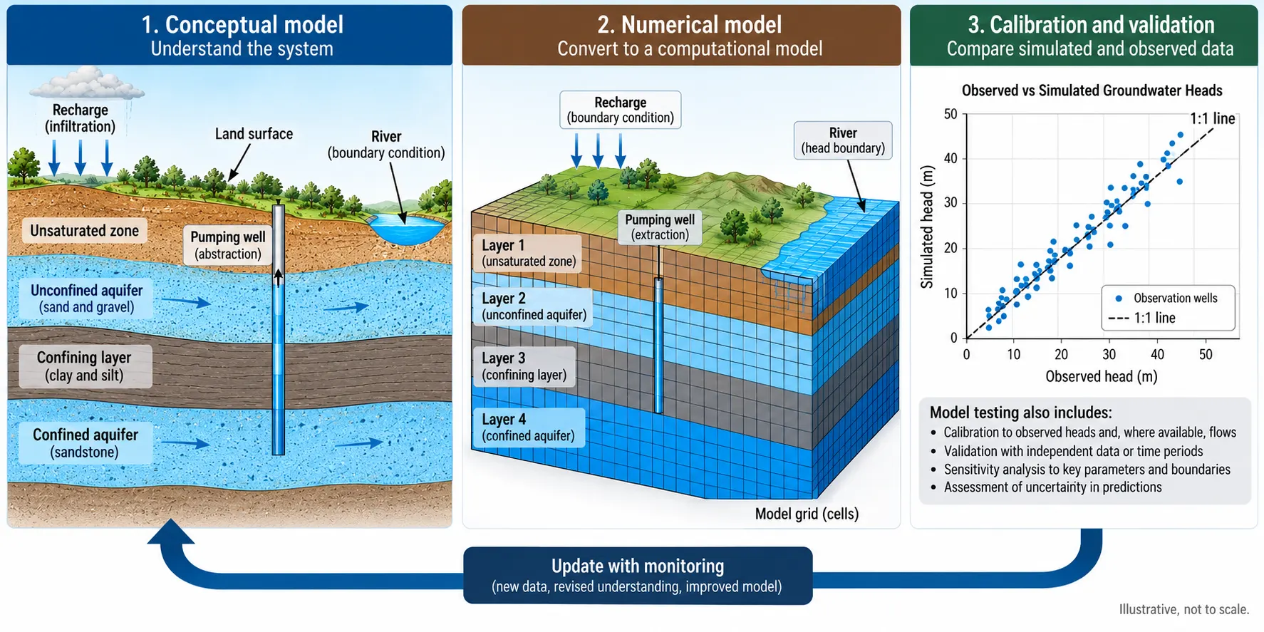
Models help with questions observation alone cannot answer, such as the effect of doubling abstraction on neighbouring wells or the reach of dewatering drawdown. A model is calibrated by adjusting uncertain parameters until simulated heads and flows match measurements. Sensitivity analysis then shows which parameters control the answer, and therefore where further investigation would be most useful.
USGS notes that model forecasts are imprecise, limited by sparse or inaccurate data, poorly defined stresses and errors in conceptualising the system, but may still be the best decision-making information available at the time. It recommends continued monitoring and periodic re-evaluation of models used for long-term questions (USGS Circular 1186). A model is a decision-support tool, not a guarantee. A predictive groundwater model is most useful when the investigation data behind it are strong enough to constrain it.
Assessing an Aquifer Before a Major Investment
When a site is being bought, a plant expanded or a deep basement approved, the aim is not to know everything about the aquifer but enough to decide, and to understand what remains uncertain.
Aquifer concerns by industry
| Sector | Typical aquifer concern | Possible consequence | Investigation usually needed |
|---|---|---|---|
| Commercial real estate | Pressure and inflow beneath basements | Delay, redesign, neighbour claims | Piezometric head, uplift and dewatering assessment |
| Manufacturing | Long-term supply, permit conditions | Production constraints | Pumping tests, interference and capture analysis |
| Data centres | Cooling supply, deep plant rooms | Supply shortfall, construction risk | Supply and excavation assessment |
| Mining | Pit inflow, dewatering effects | Operating cost, regulatory issues | Hydrogeological model, monitoring network |
| Industrial parks | Shared aquifer, cumulative abstraction | Underperforming wells, tenant disputes | Regional assessment, coordinated monitoring |
| Logistics and warehousing | Shallow groundwater, contamination liability | Foundation issues, remediation cost | Shallow investigation, baseline quality |
| Infrastructure and transport | Tunnels and linear works crossing aquifers | Inflow, settlement, programme risk | Multi-unit piezometry, settlement assessment |
| Institutional campuses | Supply resilience, recharge commitments | Supply gaps | Supply and recharge feasibility |
Regulation in India, the United States and Abu Dhabi
Regulation varies by jurisdiction and changes over time, so confirm current requirements with the regulator.
In India, the Central Ground Water Authority's guidelines were notified on 24 September 2020 as S.O. 3289(E) and required industries abstracting more than 100 m³/day to carry out an annual water audit. An amendment of 29 March 2023, S.O. 1509(E), changed this to a biennial audit, once every two years, through certified auditors of agencies approved by CGWA (CGWA Water Audit SOP, August 2024).
In the United States, groundwater is largely regulated at state and local level. In Texas, the Harris-Galveston Subsidence District requires permits for most wells before drilling or operation and limits groundwater to a set share of total water demand in each regulatory area (HGSD). California's Sustainable Groundwater Management Act of 2014 addresses six undesirable results: lowering of groundwater levels, reduction of storage, seawater intrusion, degraded quality, land subsidence and depletion of interconnected surface water (California State Water Resources Control Board).
In Abu Dhabi, Law No. 5 of 2016 establishes groundwater as government property, with the Environment Agency Abu Dhabi responsible for licensing wells, supervising drilling and setting abstraction amounts (ECOLEX summary).
A staged assessment
Investigation is most efficient when each stage informs whether, and how, to fund the next.
- Desk study of geology, boreholes, water-level trends, regulation and neighbouring users.
- Reconnaissance, including a survey of existing wells and targeted geophysics.
- Drilling and testing, with multi-depth piezometers, pumping tests and sampling.
- Analysis and modelling of supply and construction scenarios, with stated uncertainty.
- Monitoring, from a pre-development baseline onwards.
Scope depends on the project and the geology. A modest supply from well-documented alluvium needs far less than a deep basement above a confined aquifer.
| Checklist item | Evidence to look for | Warning sign |
|---|---|---|
| Aquifer type and geometry | Logs, cross-sections, regional maps | One borehole, or geology inferred from distant data |
| Heads | Multi-season records in each unit | A single reading, or none below formation level |
| Hydraulic properties | Pumping tests with observation wells | Values taken only from textbook tables |
| Abstraction history | Records of local and neighbouring pumping | Many unregistered wells nearby |
| Water quality | Recent sampling of the target unit | No baseline before development |
| Recharge and capture | Recharge estimates, links to surface water | Supply justified by rainfall alone |
| Construction risk | Uplift, inflow and settlement assessment | Basement design based on water table depth only |
| Regulation | Current permits, area classification, audit duties | Assumed approvals |
| Data gaps | Stated uncertainty and next steps | A firm conclusion with no stated uncertainty |
Frequently Asked Questions
Can an aquifer reliably supply an industrial facility?
It can, but reliability has to be demonstrated rather than assumed. Short tests show what a well can do now. Long-term reliability depends on capture, boundaries and neighbouring abstraction over the life of the facility.
Why can a site have groundwater but low well yield?
Holding water and releasing it are different properties. Clays can have high total porosity but low effective porosity, and in hard rock yield depends on whether the borehole meets connected fractures.
How long should a pumping test run?
Long enough to show the effects of the proposed pumping and any boundaries that matter for the decision, followed by recovery monitoring. Some regulators set minimum durations, so check local requirements.
Are confined aquifers always a hazard for basements?
No. The risk depends on the piezometric head, the thickness and properties of the soil above the confined layer and the excavation geometry. Many confined aquifers pose no uplift risk to a given excavation. Measured heads and a code-based check decide the question.
What should developers check about aquifers before buying land?
Aquifer type and geometry, heads in each unit, hydraulic properties, existing abstraction, water quality, recharge, construction risks and current regulation. The checklist in the previous section sets out the evidence and warning signs for each.